Using Powershell and Excel to compare Microsoft Hotfixs on Servers and Virtual Machines.

Hello All,

 

Two Types of Comparisons Devised

I have been working several Clustering and Hyper-V cases Recently.  I have come to a point where I notice the Virtual Machines rarely have the same level of  Microsoft Updates that the Cluster Node does. I finally had a few minutes to look at this issue, and I even made an Excel Spreadsheet to compare updates to other machines.

Fortunately, When I got serious about making a Spread Sheet Script, I noticed there were some pretty good work already available. In fact, I found one that will likely serve to compare updates on all the Nodes, all the VMs and more. I am sure I can do cross checks using a Host as the standard, and a bunch of VM’S as the comparisons.

So we are basically showing off two different ways of doing the same thing.  The Gallery script vs. MyExcelHotfixCompare. These are different things for different reasons. But its good to have them in the same place, Because they both have their own purpose.

 

 

First thing you want to do have is a copy of the spread sheet, MYexcelHotfixCompare , and a copy of the The Gallery script

 

Why Two Comparisons

So I made one up, and I found the other by accident! That is true. However, I discovered these both served different purposes.

The First method came from Stane Monsik. What this count does, is aggregate the KB’s for every server in the survey. So your Final report answers the question “when you updated Server Group X with KB Group Summation(A-Z), did you do that same thing to all the other servers? This is what I started out to have answered! If the answer to this is no, then I always tell my customer to finish his updates right away.

However, another question I was often asking, was not being answered by this script. The Questions was, When we know that there are X updates packages for Technology Y, how many of those updates did you apply to your server? Then Question #2,  For X and Y, did you apply these updates to just the server which had problems? The answer to this question should be that you updated all the servers which contained technology Y, with every Update Package X. I found this question was often met with Guesstimates more than actual proof; this was an easy question to get a good guess on. It’s also an easy question to just accept the guess and move on.  In today’s complex world, that is no longer acceptable. So I set out to easily answer this kind of question.

 

Method1 Script

This script will take “a list of Machines” and show you what updates the entire list has and does not have. Every KB gets added to the list, no matter what server it was found on.

The Script, located at Gallery.Tech.net.Microsoft.Com , Goes to every server and pulls the list of hot fixes. Then it goes through the hot fix list and checks every computer, to see if the hot fix has been applied to the computer.

To make GetHotfixCompare_Gallery work, all you have to do is open the .PS1 file with notepad and add your list of computer names. You can add as many computers as you like, but realize it takes longer and longer and longer to complete. The text you are editing looks like this in the file:  See Figure 1. :

# —————————————————————————————————-

$computers = “ComputerName1”, “ComputerName2”, “ComputerName3”, “ComputerName4”, “ComputerName5”

# —————————————————————————————————-

The Result is a very nice HTML report:

 

Figure 1.

 

Once you populate the script with edits on the names of computers, you run the PS1 file by right Clicking the file and choosing Run With Power Shell. The Script runs (longer the more computers you select), then generates an HTML file of your KB’s. There is an orderly chart of stars telling you which KB’s have stars for the machine, and which do not have stars.

 

All in all, A  very good method. But in order for me to answer the technology related questions, I needed to use something different.

 

Method 2 Spread Sheet comparison (MY_excel_GetHotfixCompare)

On the Excel Help article, called “Compare two lists and highlight matches and differences” I use Example 4 of that section. Example 4 runs a comparison from column one (the update list of a server (get-hotfix)  against column two (the list of updates for the specific technology) .  The comparison Colorizes the two list columns to highlight where the updates match or are unique.

MY_ExcelGetHotfixCompare Is the name of the spread, and you just need to right click and save as to save the file as an XLSX file.

This method will always work, as long as you can find a list of key updates, Microsoft says is relevant. This list below is not unabridged. This is just areas where I work most often. Below are some Example Technology Patch lists, that will power column two, on your spread sheets.

• Hyper-V updates 2012 R2
• Server 2012 Cluster Updates
• 2012 R2 Network Virtualization
• Skype Client 2016
• Exchange 2013 and 2016
• Server 2012 R2

Server 2012 and Exchange make you dig a little bit to get the actual KB list, but you get the Idea. The point is to get the list of “important hotfixes” and be able to use them to “audit” you current situation. So let’s get to the formulas and make a spread sheet!

 

Get Hot-fix Compare Spread Sheet

The Compare column Colorizes numbers in column A , that are also in column B. And Vice Versa. So there is only one caveat to this method. If the KB shows up twice in the same column, then the cell becomes colored, denoting that the patch has a match. But, This is an impossibility of the get-hot fix command. As long as your pasting in get-Hotfix results from only one machine per column, you will get a valid result. So the limitation of this, or any tool reviewing hot-fixes; don’t try to do two machines in one spread.

Steps to create:

1. Open Excel and put your Values for Get-Hotfix (just the KB) into column 1.
2. Copy the Hot-fix numbers for the relevant Microsoft KB numbers from your articles like above, into Column 2.
3. With Excel at the Home Tab, Choose “Conditional Formatting” and Manage Rules . You will see a pop up window, New Formatting rule: (figure Below)

 

 

4. Choose New Rule and “Format only unique or duplicate values”
5. There is a little Drop down that says Duplicate or Unique- You will make that choice here

 

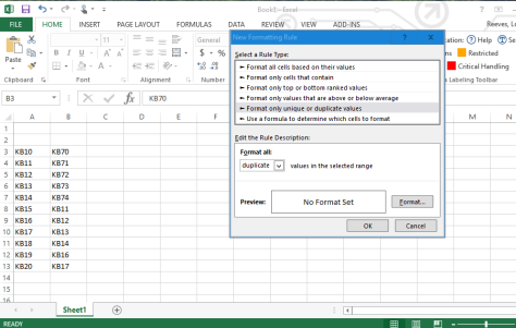
6.Then you see where it says no format set? (above) This is where you choose your color.

7. Hit the Format button. Then choose the Fill tab.

8. Now see the Fill tab below Choose your color and hit Ok.

 

9 Then Choose OK Below

 

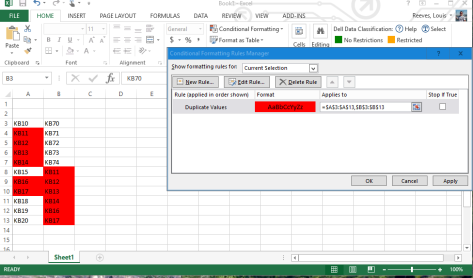
10. Now Comes the important part. You simply highlight all values in both columns and there is a wizard that will form the formula for you based on how many rows each column has in it. I am showing the screenshot below, after I clicked into the “applies to field” and held down the left click of the mouse while I selected both columns and went down enough rows to cover all values in both columns. I also found that if you pre-select both columns, before clicking conditional format, then these vales will be there automatically

11.  The only thing you can’t see in the picture above is the dashed line that is now hovering over both columns. Once I hit OK or apply, it all goes away and my formula is:

=$A$3:$B$13

Pre-Select your columns before you start with Conditional formatting

Now I found out some weirdness about the formula. If you have to go back and change the length of the column, you have to make the formula a little differently.  You click into the applies to field

and highlight Column one, then you type a comma, and then you highlight column 2. So the formula looks like this

=$A$3:$A$13,$B$3:$B$13

The more general solution is coming up below:

=$A:$A,$B:$B

I like the second formula better, because you can see the start and finish of each column. But the more general one covers all KB in both Columns. cant beat that. I am editing this sentence,

after the fact, and I found that if you select the columns, by Highlighting the columns entirely, you don’t have to deal with touching any formula aspect at  all.

Here the download again for My Excel HotfixCompare , You can also watch the video at the top and make your own spread.

Believe it or not, that is it! When you hit OK, your values immediately calculate out:

 

The next issue I tried to solve was the length of the column. It looks to me that this is the master formula, no matter how many KB s you have  (=$A:$A,$B:$B). This is for column A and B.

I do believe you could replace these values with columns a and c or b and E or whatever. This can help you move columns for your ease of use and you list can be as long or short as you want.

So use this in your Duplicate Values formula:

=$A:$A,$B:$B

Again, I am coming back after the fact, and just saying to Highlight the columns you want to use, before you start, and you don’t have to deal with the formulas at all. I have a second Excel

Method for comparing up to 6 servers, but I will let you just download the Excel File and see how it works!!! Watch the video, I performed that in about 1 minute in the video. also

after the fact, and I found that if you select the columns, by Highlighting the columns entirely, you don’t have to deal with touching any formula aspect at  all.

 

How do I get my Hot-fix list = Get-Hotfix

So this is all we have left to cover. Below these are the steps I use to get that list of KB numbers isolated from the rest of the information you find when you run the Get-Hotfix command.

 

1. Open PowerShell as Administrator

2. You may run Get-Hotfix > c:\myhotfix.txt

3. Open Notepad ++ and Open myhotfix.txt

4. Hold Control and Alt Key on your keyboard at the same time

5. While (4) use the mouse to select just the KB column

6. once the KBs are highlighted Right click and choose copy.

7. Paste you KBs into notepad for transport to your work station.

That’s It! I hope you have enjoyed this article. In closing I have the original link for the script in the initial discussion. I also have a method to update your Hyper-V Cluster automatically with a script. That can be pretty handy.